Week 4 of Neural Networks and Deep Learning
Deep Neural Network
Deep L-layer neural network
Video #1 says that a deep neural network has 1+ hidden layers. The more layers, the deeper. Deep nets can solve problems that shallow nets just can’t. It recaps some notation from the previous week.
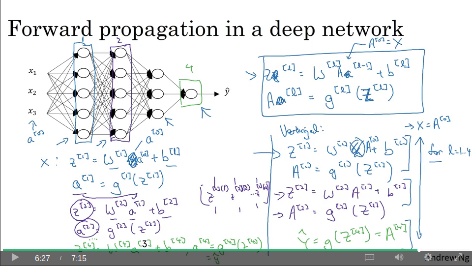
Forward propagation in a deep neural network
Video #2 shows what forward prop looks like in a deep net. Ng notes that a foor-loop would be necessary when applying Z = WA + b for each layer, so vectorisation can’t be applied here.
Getting your matrix dimensions right
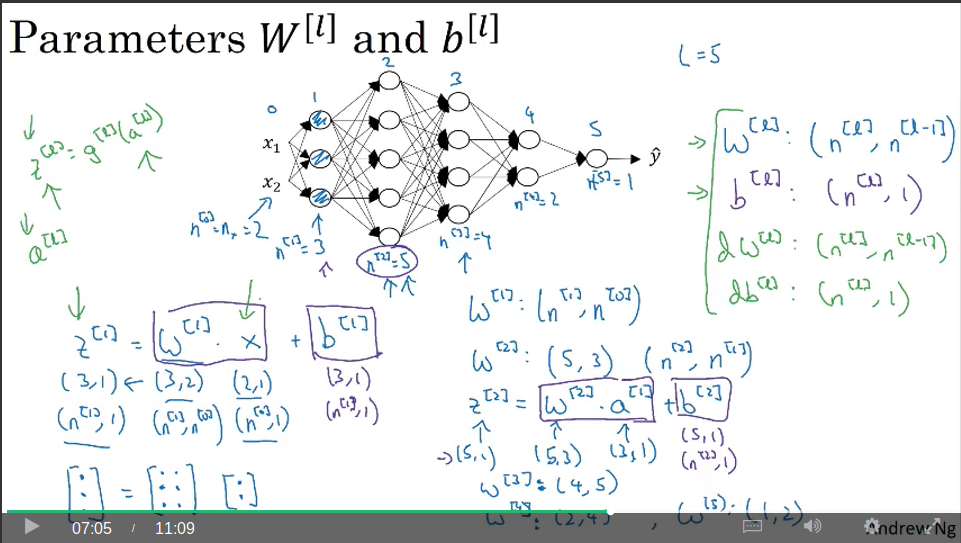
Video #3 says a nice way to ensure your model is bug-free is asserting the matrix dimensions are correct through-out.
For a hidden layer of weights, the dimension would be Wl = (nl , nl-1) A hidden layer bias vector would be bl = (nl, 1) The derivatives of w and b would have the same dimensions.
For Z = WX + b we have: (n1, 1) = (n1, n0) . (n0, 1) + (n1, 1)
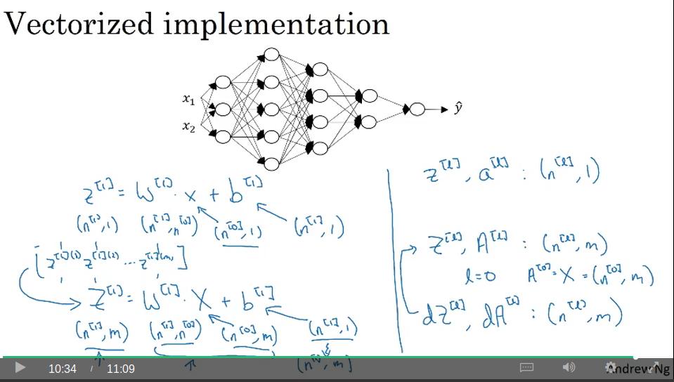
And vectorised:
For Z = WX + b we have: (n1, m) = (n1, n0) . (n0, m) + (n1, 1) and then the b vector becomes (n1,m) thanks to Python broadcasting.
Why deep representations?
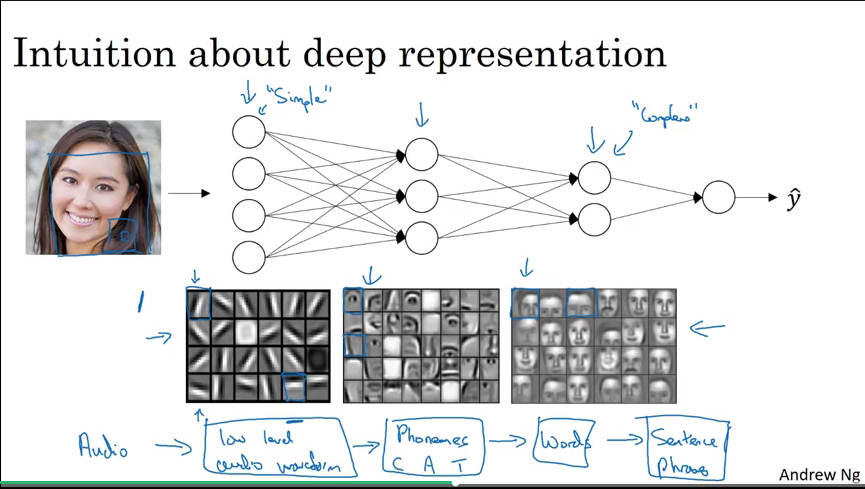
Video #4 provides some intuition as to why deep nets are better than shallow nets for some problems.
Going from left to right through the hidden layers, the left layer would detect small features like vertical or horizontal lines. The next layer might combine these lines and use them as building blocks for detecting larger features, like an eye or a nose. The next layer goes further by combining eyes and noses into faces.
(as an aside, this is where Capsule Networks make networks better in the sense that an eye a nose in a certain configuration can vote about what the surrounding face is, whereas currently a neural net would still classify a face as a face if you swap a face’s nose and mouth, for instance.)
Ng also mentions a result from circuit theory, but he doesn’t find the result very useful for intuiting about the usefulness of deep VS shallow nets, so I won’t note it here.
Building blocks of deep neural networks
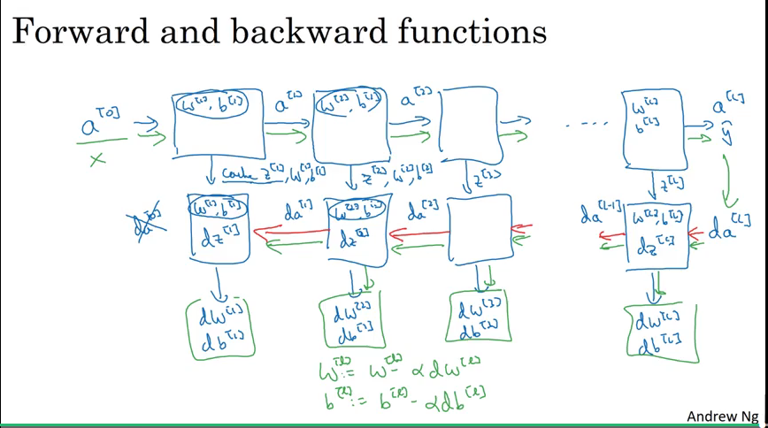
Video #5 shows the building blocks, which is basically the single layer stuff from the previous week, but extrapolated out over l1, l2, …, ln.
Forward and backward propagation
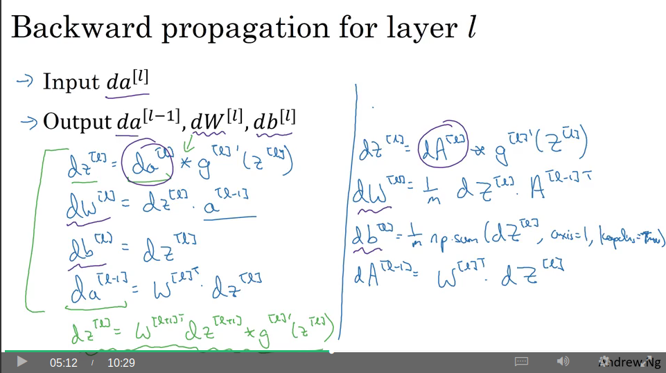
Video #6 discusses implementing the steps from the previous videos.
Again, it’s the formulas from the previous week, but extrapolated over layers l1, l2, …, ln. (the un-avoidable for-loop)
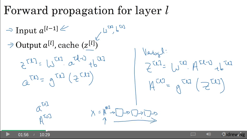
Forward
Backward
Summary
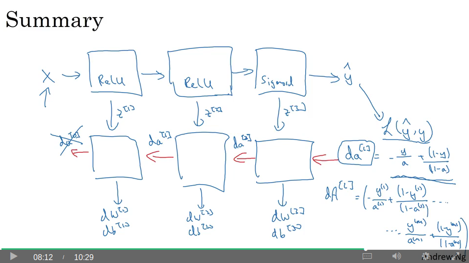
As X is the input for forward, what is the input for backward? This would be the derivative of the loss, L(yhat, y), which can be shown to be dal = -y/a + (1-y)/(1-a) but for the vectorised version dAl.
Parameters VS Hyperparameters
Video #7 says that parameters are W and b. Hyperparameters are learning rate, iterations, number of hiden layers, number of hidden units per layer. choice of activation function, etc.
Later: momentum term, minibatch size, regularisation parameters, etc.
Applied deep learning is a very empirical process.
It’s difficult to know the best configuration in advance, so iterate a lot. You can build a sense of hyperparameters across applications.
Also, what works today might not apply to tomorrow. E.g. GPUs change, inputs change.
Active area of research.
What does this have to do with the brain?
Video #8 says the answer is “not a whole lot”. Shows an analogy between a single logistical unit and a biological neuron.
Things to look forward to
In the next course
- Tuning hyper-parameters, and iterating models
- Regularisation
- Early stopping, and optimisation
During the exams, when training models some models had worse results when too many iterations were used. Lower iterations gives better accuracy on the test set. This is called “early stopping”. Early stopping is a way to prevent overfitting.
And… we’ll be learning Tensorflow. Being a dual-Clojure/Python dev, I’ve actually spent most of my time with Cortex, so I’m excited to expand my toolbox.
References in exam:
http://stackoverflow.com/questions/1907993/autoreload-of-modules-in-ipython
And that wraps up the first course.
